2024. 1. 4. 17:25ㆍData Science/Study 자료
날짜 자동 생성
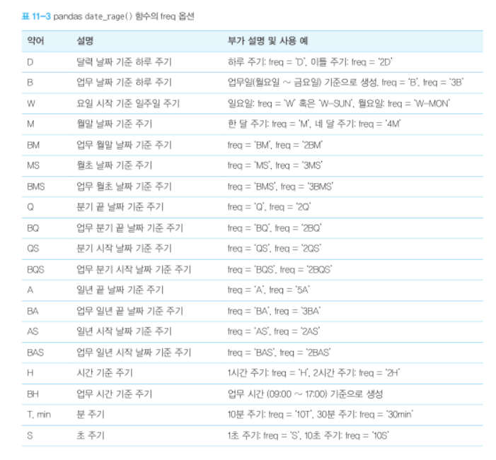
pandas_data_range()함수의 freq 옵션
Time series / date functionality — pandas 2.1.4 documentation
Time series / date functionality pandas contains extensive capabilities and features for working with time series data for all domains. Using the NumPy datetime64 and timedelta64 dtypes, pandas has consolidated a large number of features from other Python
pandas.pydata.org
https://pandas.pydata.org/docs/user_guide/timeseries.html#timeseries-offset-aliases
Time series / date functionality — pandas 2.1.4 documentation
Time series / date functionality pandas contains extensive capabilities and features for working with time series data for all domains. Using the NumPy datetime64 and timedelta64 dtypes, pandas has consolidated a large number of features from other Python
pandas.pydata.org
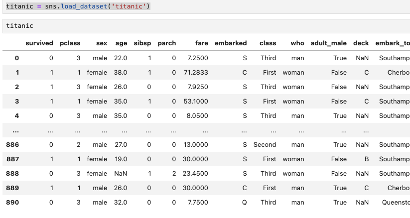
샘플 데이터셋의 종류를 알아보고 titanic 데이터 셋을 불러와보았다.
DataFrame에서 필터링
- 조건식을 통해서 필터링이 된다
- 불린을 이용하여 필터링 후 True값만 출력이 되도록 하는 작업
위와 동일한 방법으로 loc 명령어를 사용하여 'embark_town'이 'Southampton'인 데이터만 추출을 해보았다.

핵심 코드는
titanic.loc[titanic['칼럼명'] == '항목명', 인덱스번호]
인덱스번호 대신 ':'을 쓰면 전체 인덱스를 선택할 수 있다
다중 조건문 추출
and 연산자의 경우 tips.loc[(조건1) & (조건2),:]
or 연산자의 경우 tips.loc[(조건1) | (조건2),:]
다중 조건문 Tip
.loc[
,:]
사전형태와 같이 써주면 실수를 방지할 수 있음
예시)
tips.loc[
(tips['tip'] > 2.998279) &
(tips['time'] == 'Dinner')&
(tips['size'] == 3) &
(tips['sex'] == 'Male') &
(tips['day'] == 'Sat')
, :] #이러한 형태가 안헷갈림
공부 코드
import pandas as pd
import numpy as np
pd.__version__
'2.1.4'pandas 데이터 구조
- Series 데이터 구조 1차원 데이터 : 컬럼의 갯수가 1개인 데이터
- DataFrame 데이터 구조 컬럼 갯수가 여러개인 데이터
s1 = pd.Series([10, 20, 30, 40, 50])
s1 #가장 왼쪽 인덱스 타입은 정수로 처리
0    10
1    20
2    30
3    40
4    50
dtype: int64s1.index
RangeIndex(start=0, stop=5, step=1)s1.values #넘파이 배열
array([10, 20, 30, 40, 50])s2 = pd.Series(['a','b','c',1,2,3])
s2 #object로 처리 간단하게 말하면 문자로 처리
0    a
1    b
2    c
3    1
4    2
5    3
dtype: objects3 = pd.Series([np.nan,10,30]) # nan은 결측치(missing value)
s3
0     NaN
1    10.0
2    30.0
dtype: float64index_date = ['2018-10-07','2018-10-10'] # 인덱스에 데이터를 넣는것이 가능
s4 = pd.Series([200, 195],index = index_date)# 명령어
s4
2018-10-07    200
2018-10-10    195
dtype: int64index_date = ['2018-10-08','2018-10-10'] # 인덱스에 데이터를 넣는것이 가능
s4 = pd.Series([200, 195],index = index_date)# 명령어
s4
#코드상으로는 중복이 가능하지만 인덱스의 기본원칙은 충복이 되면 안됨
2018-10-08    200
2018-10-10    195
dtype: int64data_dict = {
'국어' : 100,
'영어' : 95
}
s5 = pd.Series(data_dict)
s5
국어 100
영어 95
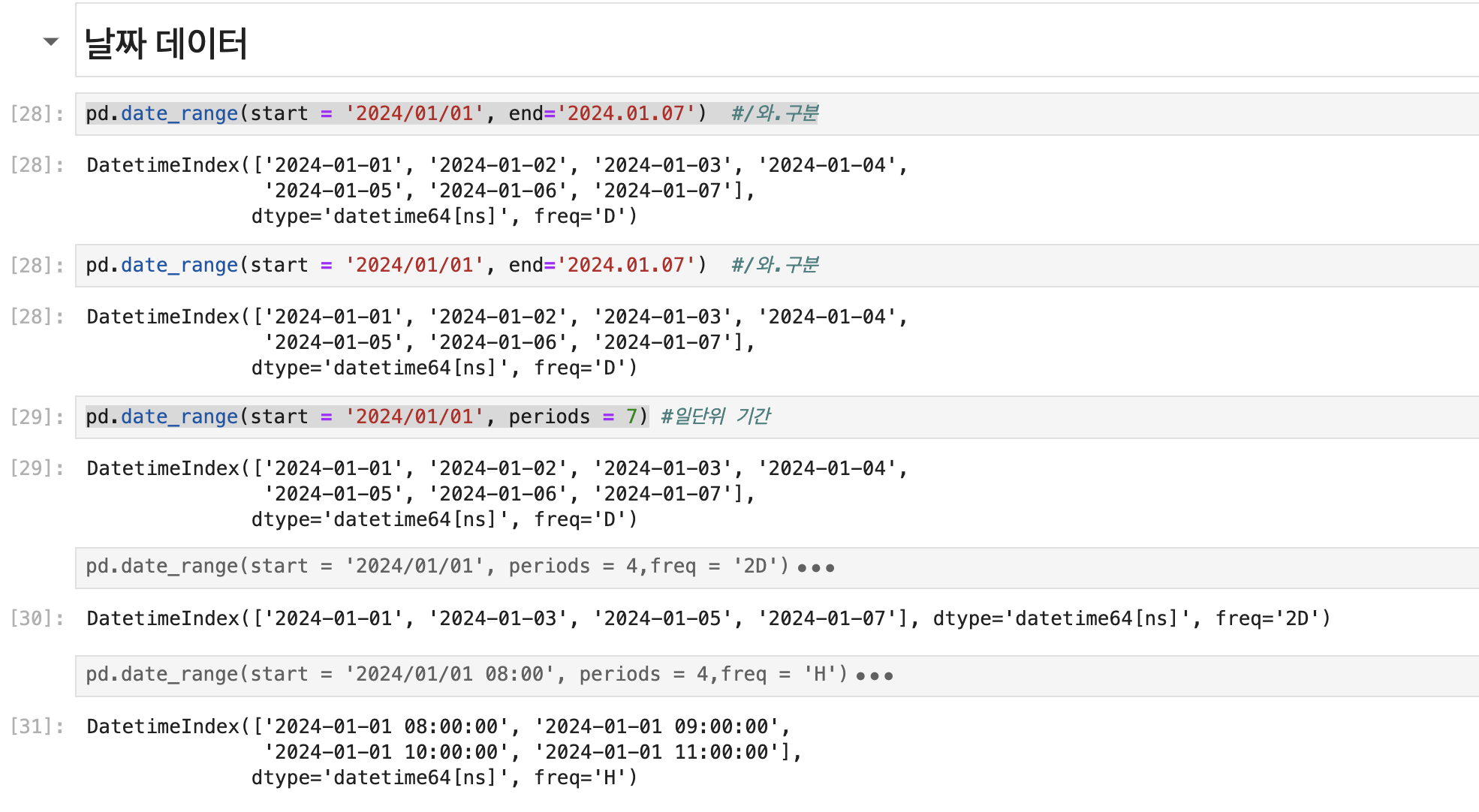
dtype: int64날짜 데이터
pd.date_range(start = '2024/01/01', end='2024.01.07') #/와.구분
DatetimeIndex(['2024-01-01', '2024-01-02', '2024-01-03', '2024-01-04',
               '2024-01-05', '2024-01-06', '2024-01-07'],
dtype='datetime64[ns]', freq='D')pd.date_range(start = '2024/01/01', end='2024.01.07') #/와.구분
DatetimeIndex(['2024-01-01', '2024-01-02', '2024-01-03', '2024-01-04',
               '2024-01-05', '2024-01-06', '2024-01-07'],
dtype='datetime64[ns]', freq='D')pd.date_range(start = '2024/01/01', periods = 7) #일단위 기간
DatetimeIndex(['2024-01-01', '2024-01-02', '2024-01-03', '2024-01-04',
               '2024-01-05', '2024-01-06', '2024-01-07'],
dtype='datetime64[ns]', freq='D')pd.date_range(start = '2024/01/01', periods = 4,freq = '2D')
DatetimeIndex(['2024-01-01', '2024-01-03', '2024-01-05', '2024-01-07'], dtype='datetime64[ns]', freq='2D')pd.date_range(start = '2024/01/01 08:00', periods = 4,freq = 'H')
DatetimeIndex(['2024-01-01 08:00:00', '2024-01-01 09:00:00',
               '2024-01-01 10:00:00', '2024-01-01 11:00:00'],
              dtype='datetime64[ns]', freq='H')
DataFrame을 활용한 데이터 생성
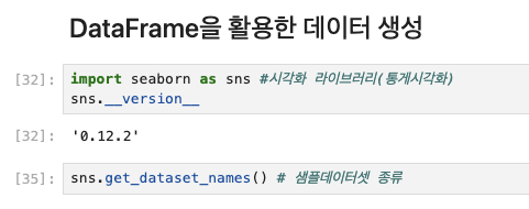
import seaborn as sns #시각화 라이브러리(통게시각화)
sns.__version__
'0.12.2'sns.get_dataset_names() # 샘플데이터셋 종류
['anagrams',
 'anscombe',
 'attention',
 'brain_networks',
 'car_crashes',
 'diamonds',
 'dots',
 'dowjones',
 'exercise',
 'flights',
 'fmri',
 'geyser',
 'glue',
 'healthexp',
 'iris',
 'mpg',
 'penguins',
 'planets',
 'seaice',
 'taxis',
 'tips',
'titanic']iris = sns.load_dataset('iris')
iris
| 5.1 | 3.5 | 1.4 | 0.2 | setosa |
| 4.9 | 3.0 | 1.4 | 0.2 | setosa |
| 4.7 | 3.2 | 1.3 | 0.2 | setosa |
| 4.6 | 3.1 | 1.5 | 0.2 | setosa |
| 5.0 | 3.6 | 1.4 | 0.2 | setosa |
| ... | ... | ... | ... | ... |
| 6.7 | 3.0 | 5.2 | 2.3 | virginica |
| 6.3 | 2.5 | 5.0 | 1.9 | virginica |
| 6.5 | 3.0 | 5.2 | 2.0 | virginica |
| 6.2 | 3.4 | 5.4 | 2.3 | virginica |
| 5.9 | 3.0 | 5.1 | 1.8 | virginica |
150 rows × 5 columns
#247p 참고
#249p 딕셔너리 스타일 좋아함
table_data = {
'연도' : [2015, 2016, 2016, 2017, 2017],
'지사' : ['한국', '한국', '미국', '한국', '미국'],
'고객수' : [200,250,450,300,500]
}
data = pd.DataFrame(table_data)
table_data
{'연도': [2015, 2016, 2016, 2017, 2017],
'지사': ['한국', '한국', '미국', '한국', '미국'],
'고객수': [200, 250, 450, 300, 500]}data.index
RangeIndex(start=0, stop=5, step=1)data.values #차원확인 .shape
array([[2015, '한국', 200],
[2016, '한국', 250],
[2016, '미국', 450],
[2017, '한국', 300],
[2017, '미국', 500]], dtype=object)- 데이터 가공 시,numpy 메서드와 pandas 메서드 조합을 해서 처리하는 경우 많음
- vectorization으로 처리/ 파이썬 기초문법(for-loop) 대신
- 속도가 매우빠름 (gpt처리도 괜찮음)
data.columns
Index(['연도', '지사', '고객수'], dtype='object')titanic = sns.load_dataset('titanic')
titanic
| 0 | 3 | male | 22.0 | 1 | 0 | 7.2500 | S | Third | man | True | NaN | Southampton | no | False |
| 1 | 1 | female | 38.0 | 1 | 0 | 71.2833 | C | First | woman | False | C | Cherbourg | yes | False |
| 1 | 3 | female | 26.0 | 0 | 0 | 7.9250 | S | Third | woman | False | NaN | Southampton | yes | True |
| 1 | 1 | female | 35.0 | 1 | 0 | 53.1000 | S | First | woman | False | C | Southampton | yes | False |
| 0 | 3 | male | 35.0 | 0 | 0 | 8.0500 | S | Third | man | True | NaN | Southampton | no | True |
| ... | ... | ... | ... | ... | ... | ... | ... | ... | ... | ... | ... | ... | ... | ... |
| 0 | 2 | male | 27.0 | 0 | 0 | 13.0000 | S | Second | man | True | NaN | Southampton | no | True |
| 1 | 1 | female | 19.0 | 0 | 0 | 30.0000 | S | First | woman | False | B | Southampton | yes | True |
| 0 | 3 | female | NaN | 1 | 2 | 23.4500 | S | Third | woman | False | NaN | Southampton | no | False |
| 1 | 1 | male | 26.0 | 0 | 0 | 30.0000 | C | First | man | True | C | Cherbourg | yes | True |
| 0 | 3 | male | 32.0 | 0 | 0 | 7.7500 | Q | Third | man | True | NaN | Queenstown | no | True |
891 rows × 15 columns
titanic.head()
| 0 | 3 | male | 22.0 | 1 | 0 | 7.2500 | S | Third | man | True | NaN | Southampton | no | False |
| 1 | 1 | female | 38.0 | 1 | 0 | 71.2833 | C | First | woman | False | C | Cherbourg | yes | False |
| 1 | 3 | female | 26.0 | 0 | 0 | 7.9250 | S | Third | woman | False | NaN | Southampton | yes | True |
| 1 | 1 | female | 35.0 | 1 | 0 | 53.1000 | S | First | woman | False | C | Southampton | yes | False |
| 0 | 3 | male | 35.0 | 0 | 0 | 8.0500 | S | Third | man | True | NaN | Southampton | no | True |
DataFrame에서 열 선택
age = titanic['age']
age.head()
0 22.0
1 38.0
2 26.0
3 35.0
4 35.0
Name: age, dtype: float64type(titanic['age'])
pandas.core.series.Seriesage_sex = titanic[['age','sex']]
age_sex
| 22.0 | male |
| 38.0 | female |
| 26.0 | female |
| 35.0 | female |
| 35.0 | male |
| ... | ... |
| 27.0 | male |
| 19.0 | female |
| NaN | female |
| 26.0 | male |
| 32.0 | male |
891 rows × 2 columns
type(titanic[['age','sex']])
pandas.core.frame.DataFrametitanic[['age','sex']].shape
(891, 2)DataFrame에서 행 필터링
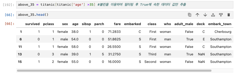
- 조건식을 통해서 필터링이 됨
above_35 = titanic[titanic['age'] >35] #불린을 이용하여 필터링 후 True에 속한 데이터 값만 추출
above_35.head()
| 1 | 1 | female | 38.0 | 1 | 0 | 71.2833 | C | First | woman | False | C | Cherbourg | yes | False |
| 0 | 1 | male | 54.0 | 0 | 0 | 51.8625 | S | First | man | True | E | Southampton | no | True |
| 1 | 1 | female | 58.0 | 0 | 0 | 26.5500 | S | First | woman | False | C | Southampton | yes | True |
| 0 | 3 | male | 39.0 | 1 | 5 | 31.2750 | S | Third | man | True | NaN | Southampton | no | False |
| 1 | 2 | female | 55.0 | 0 | 0 | 16.0000 | S | Second | woman | False | NaN | Southampton | yes | True |
above_35.shape
(217, 15)# 객실 2,3만 보고싶음
class_23 = titanic[titanic['pclass'].isin([2, 3])]
class_23.head()
| 0 | 3 | male | 22.0 | 1 | 0 | 7.2500 | S | Third | man | True | NaN | Southampton | no | False |
| 1 | 3 | female | 26.0 | 0 | 0 | 7.9250 | S | Third | woman | False | NaN | Southampton | yes | True |
| 0 | 3 | male | 35.0 | 0 | 0 | 8.0500 | S | Third | man | True | NaN | Southampton | no | True |
| 0 | 3 | male | NaN | 0 | 0 | 8.4583 | Q | Third | man | True | NaN | Queenstown | no | True |
| 0 | 3 | male | 2.0 | 3 | 1 | 21.0750 | S | Third | child | False | NaN | Southampton | no | False |
class_23 = titanic[(titanic["pclass"] == 2) | (titanic["pclass"] == 3)]
class_23.head()
| 0 | 3 | male | 22.0 | 1 | 0 | 7.2500 | S | Third | man | True | NaN | Southampton | no | False |
| 1 | 3 | female | 26.0 | 0 | 0 | 7.9250 | S | Third | woman | False | NaN | Southampton | yes | True |
| 0 | 3 | male | 35.0 | 0 | 0 | 8.0500 | S | Third | man | True | NaN | Southampton | no | True |
| 0 | 3 | male | NaN | 0 | 0 | 8.4583 | Q | Third | man | True | NaN | Queenstown | no | True |
| 0 | 3 | male | 2.0 | 3 | 1 | 21.0750 | S | Third | child | False | NaN | Southampton | no | False |
#.isin() 명령어는 or연산자(|)와 같은 역할을 한다
#나이가 적힌 데이터만 추출
titanic['age'].notna() #나이에 결측값이 있는 사람을 필터링
0 True
1 True
2 True
3 True
4 True
...
886 True
887 True
888 False
889 True
890 True
Name: age, Length: 891, dtype: booltitanic[titanic['age'].notna()] #불린값으로 받은 데이터자료
| 0 | 3 | male | 22.0 | 1 | 0 | 7.2500 | S | Third | man | True | NaN | Southampton | no | False |
| 1 | 1 | female | 38.0 | 1 | 0 | 71.2833 | C | First | woman | False | C | Cherbourg | yes | False |
| 1 | 3 | female | 26.0 | 0 | 0 | 7.9250 | S | Third | woman | False | NaN | Southampton | yes | True |
| 1 | 1 | female | 35.0 | 1 | 0 | 53.1000 | S | First | woman | False | C | Southampton | yes | False |
| 0 | 3 | male | 35.0 | 0 | 0 | 8.0500 | S | Third | man | True | NaN | Southampton | no | True |
| ... | ... | ... | ... | ... | ... | ... | ... | ... | ... | ... | ... | ... | ... | ... |
| 0 | 3 | female | 39.0 | 0 | 5 | 29.1250 | Q | Third | woman | False | NaN | Queenstown | no | False |
| 0 | 2 | male | 27.0 | 0 | 0 | 13.0000 | S | Second | man | True | NaN | Southampton | no | True |
| 1 | 1 | female | 19.0 | 0 | 0 | 30.0000 | S | First | woman | False | B | Southampton | yes | True |
| 1 | 1 | male | 26.0 | 0 | 0 | 30.0000 | C | First | man | True | C | Cherbourg | yes | True |
| 0 | 3 | male | 32.0 | 0 | 0 | 7.7500 | Q | Third | man | True | NaN | Queenstown | no | True |
714 rows × 15 columns
age_no_na = titanic[titanic['age'].notna()]
age_no_na.head()
| 0 | 3 | male | 22.0 | 1 | 0 | 7.2500 | S | Third | man | True | NaN | Southampton | no | False |
| 1 | 1 | female | 38.0 | 1 | 0 | 71.2833 | C | First | woman | False | C | Cherbourg | yes | False |
| 1 | 3 | female | 26.0 | 0 | 0 | 7.9250 | S | Third | woman | False | NaN | Southampton | yes | True |
| 1 | 1 | female | 35.0 | 1 | 0 | 53.1000 | S | First | woman | False | C | Southampton | yes | False |
| 0 | 3 | male | 35.0 | 0 | 0 | 8.0500 | S | Third | man | True | NaN | Southampton | no | True |
age_no_na.shape #나이 결측값이 있는 항목을 삭제한 데이터프레임
(714, 15)특정 행과 열을 선택해보기
- .loc[인덱스의 명칭 , 칼럼의 명칭]
- .iloc[인덱스번호,칼럼번호]
adult_name = titanic.loc[titanic['age'] > 35, 'embark_town']
adult_name.head()
1 Cherbourg
6 Southampton
11 Southampton
13 Southampton
15 Southampton
Name: embark_town, dtype: objecttitanic.iloc[0:3,3] = 'anonymous' # 0부터 2까지의 인덱스, 3번째 칼럼에서 의 값을 anonymous로 바꿈
titanic.head()
/var/folders/dk/vy49vgx92_3d76t7s3b_x5c40000gn/T/ipykernel_92221/253640465.py:1: FutureWarning: Setting an item of incompatible dtype is deprecated and will raise in a future error of pandas. Value 'anonymous' has dtype incompatible with float64, please explicitly cast to a compatible dtype first.
titanic.iloc[0:3,3] = 'anonymous'
| 0 | 3 | male | anonymous | 1 | 0 | 7.2500 | S | Third | man | True | NaN | Southampton | no | False |
| 1 | 1 | female | anonymous | 1 | 0 | 71.2833 | C | First | woman | False | C | Cherbourg | yes | False |
| 1 | 3 | female | anonymous | 0 | 0 | 7.9250 | S | Third | woman | False | NaN | Southampton | yes | True |
| 1 | 1 | female | 35.0 | 1 | 0 | 53.1000 | S | First | woman | False | C | Southampton | yes | False |
| 0 | 3 | male | 35.0 | 0 | 0 | 8.0500 | S | Third | man | True | NaN | Southampton | no | True |
데이터 연산
import seaborn as sns
s1 = pd.Series([1,2,3,4,5])
s2 = pd.Series([10,20,30,40,50])
s1+s2 #시리즈의 연산이 가능(-,*,/)
0 11
1 22
2 33
3 44
4 55
dtype: int64#리스트와 numpy의 배열과 다르게, 서로 크기가 달라도 연산이 가능함
s1 = pd.Series([1,2,3,4])
s2 = pd.Series([10,20,30,40,50])
s1+s2
0 11.0
1 22.0
2 33.0
3 44.0
4 NaN
dtype: float64#단 결과값은 NaN 결측치로 표기가 된다
table_data1 = {'A': [1, 2, 3, 4, 5],
'B': [10, 20, 30, 40, 50],
'C': [100, 200, 300, 400, 500]}
df1 = pd.DataFrame(table_data1)
df1
| 1 | 10 | 100 |
| 2 | 20 | 200 |
| 3 | 30 | 300 |
| 4 | 40 | 400 |
| 5 | 50 | 500 |
table_data2 = {'A': [6, 7, 8],
'B': [60, 70, 80],
'C': [600, 700, 800]}
df2 = pd.DataFrame(table_data2)
df2
| 6 | 60 | 600 |
| 7 | 70 | 700 |
| 8 | 80 | 800 |
df1 + df2
| 7.0 | 70.0 | 700.0 |
| 9.0 | 90.0 | 900.0 |
| 11.0 | 110.0 | 1100.0 |
| NaN | NaN | NaN |
| NaN | NaN | NaN |
df1 - df2
| -5.0 | -50.0 | -500.0 |
| -5.0 | -50.0 | -500.0 |
| -5.0 | -50.0 | -500.0 |
| NaN | NaN | NaN |
| NaN | NaN | NaN |
df1 * df2
| 6.0 | 600.0 | 60000.0 |
| 14.0 | 1400.0 | 140000.0 |
| 24.0 | 2400.0 | 240000.0 |
| NaN | NaN | NaN |
| NaN | NaN | NaN |
df1 / df2
| 0.166667 | 0.166667 | 0.166667 |
| 0.285714 | 0.285714 | 0.285714 |
| 0.375000 | 0.375000 | 0.375000 |
| NaN | NaN | NaN |
| NaN | NaN | NaN |
table_data3 = {'봄': [256.5, 264.3, 215.9, 223.2, 312.8],
'여름': [770.6, 567.5, 599.8, 387.1, 446.2],
'가을': [363.5, 231.2, 293.1, 247.7, 381.6],
'겨울': [139.3, 59.9, 76.9, 109.1, 108.1]}
columns_list = ['봄', '여름', '가을', '겨울']
index_list = ['2012', '2013', '2014', '2015', '2016']
df3 = pd.DataFrame(table_data3, columns = columns_list, index = index_list)
df3
| 256.5 | 770.6 | 363.5 | 139.3 |
| 264.3 | 567.5 | 231.2 | 59.9 |
| 215.9 | 599.8 | 293.1 | 76.9 |
| 223.2 | 387.1 | 247.7 | 109.1 |
| 312.8 | 446.2 | 381.6 | 108.1 |
df3.mean()
봄 254.54
여름 554.24
가을 303.42
겨울 98.66
dtype: float64df3.max()
봄 312.8
여름 770.6
가을 381.6
겨울 139.3
dtype: float64df3.min()
봄 215.9
여름 387.1
가을 231.2
겨울 59.9
dtype: float64df3.mean(axis=1) #행으로 평균을 냄 axis=1
2012 382.475
2013 280.725
2014 296.425
2015 241.775
2016 312.175
dtype: float64df3.max(axis=1)
2012 770.6
2013 567.5
2014 599.8
2015 387.1
2016 446.2
dtype: float64df3.std(axis=1) #행단위 표준편차
2012 274.472128
2013 211.128782
2014 221.150739
2015 114.166760
2016 146.548658
dtype: float64해석하는 능력을 키워야함
- 평균을 중심으로 표준편차는 폭을 나타냄 즉 2012년도는 편차가 여름에비해 다른계절이 큼
- 2015년은 폭이 작아 여름과 비교하면 편차가 작음
- 데이터의 분포가 상상이 되야함(평균과 표준편차를보고)
df3.describe()
| 5.000000 | 5.000000 | 5.000000 | 5.000000 |
| 254.540000 | 554.240000 | 303.420000 | 98.660000 |
| 38.628267 | 148.888895 | 67.358496 | 30.925523 |
| 215.900000 | 387.100000 | 231.200000 | 59.900000 |
| 223.200000 | 446.200000 | 247.700000 | 76.900000 |
| 256.500000 | 567.500000 | 293.100000 | 108.100000 |
| 264.300000 | 599.800000 | 363.500000 | 109.100000 |
| 312.800000 | 770.600000 | 381.600000 | 139.300000 |
df3.T.describe()
| 4.000000 | 4.000000 | 4.000000 | 4.00000 | 4.000000 |
| 382.475000 | 280.725000 | 296.425000 | 241.77500 | 312.175000 |
| 274.472128 | 211.128782 | 221.150739 | 114.16676 | 146.548658 |
| 139.300000 | 59.900000 | 76.900000 | 109.10000 | 108.100000 |
| 227.200000 | 188.375000 | 181.150000 | 194.67500 | 261.625000 |
| 310.000000 | 247.750000 | 254.500000 | 235.45000 | 347.200000 |
| 465.275000 | 340.100000 | 369.775000 | 282.55000 | 397.750000 |
| 770.600000 | 567.500000 | 599.800000 | 387.10000 | 446.200000 |
KTX_data = {'경부선 KTX': [39060, 39896, 42005, 43621, 41702, 41266, 32427],
'호남선 KTX': [7313, 6967, 6873, 6626, 8675, 10622, 9228],
'경전선 KTX': [3627, 4168, 4088, 4424, 4606, 4984, 5570],
'전라선 KTX': [309, 1771, 1954, 2244, 3146, 3945, 5766],
'동해선 KTX': [np.nan,np.nan, np.nan, np.nan, 2395, 3786, 6667]}
index_list = ['2011', '2012', '2013', '2014', '2015', '2016', '2017']
df_KTX = pd.DataFrame(KTX_data, index = index_list)
df_KTX
| 39060 | 7313 | 3627 | 309 | NaN |
| 39896 | 6967 | 4168 | 1771 | NaN |
| 42005 | 6873 | 4088 | 1954 | NaN |
| 43621 | 6626 | 4424 | 2244 | NaN |
| 41702 | 8675 | 4606 | 3146 | 2395.0 |
| 41266 | 10622 | 4984 | 3945 | 3786.0 |
| 32427 | 9228 | 5570 | 5766 | 6667.0 |
#p.259
df_KTX.head(3)
| 39060 | 7313 | 3627 | 309 | NaN |
| 39896 | 6967 | 4168 | 1771 | NaN |
| 42005 | 6873 | 4088 | 1954 | NaN |
df_KTX.tail(3)
| 41702 | 8675 | 4606 | 3146 | 2395.0 |
| 41266 | 10622 | 4984 | 3945 | 3786.0 |
| 32427 | 9228 | 5570 | 5766 | 6667.0 |
행 선택 (행 추출)
- slicing과 동일한 문법으로 추출 가능
df_KTX[0:2] #인덱스 순번
| 39060 | 7313 | 3627 | 309 | NaN |
| 39896 | 6967 | 4168 | 1771 | NaN |
df_KTX[2:5]
| 42005 | 6873 | 4088 | 1954 | NaN |
| 43621 | 6626 | 4424 | 2244 | NaN |
| 41702 | 8675 | 4606 | 3146 | 2395.0 |
loc vs iloc를 활용한 열 추출, 행 추출
- 두 가지의 차이 기억하기
#df_KTX,loc[행,열]
#df_KTX.loc['2013':'2016']
| 42005 | 6873 | 4088 | 1954 | NaN |
| 43621 | 6626 | 4424 | 2244 | NaN |
| 41702 | 8675 | 4606 | 3146 | 2395.0 |
| 41266 | 10622 | 4984 | 3945 | 3786.0 |
df_KTX.loc['2013':'2016','경부선 KTX']
2013 42005
2014 43621
2015 41702
2016 41266
Name: 경부선 KTX, dtype: int64df_KTX.loc['2013':'2016',['경부선 KTX','호남선 KTX']]
| 42005 | 6873 |
| 43621 | 6626 |
| 41702 | 8675 |
| 41266 | 10622 |
df_KTX.loc['2013':'2016',['호남선 KTX']]
| 6873 |
| 6626 |
| 8675 |
| 10622 |
#외울때 df.loc[행조건식, [컬럼명]]
iris = sns.load_dataset('iris')
iris
| 5.1 | 3.5 | 1.4 | 0.2 | setosa |
| 4.9 | 3.0 | 1.4 | 0.2 | setosa |
| 4.7 | 3.2 | 1.3 | 0.2 | setosa |
| 4.6 | 3.1 | 1.5 | 0.2 | setosa |
| 5.0 | 3.6 | 1.4 | 0.2 | setosa |
| ... | ... | ... | ... | ... |
| 6.7 | 3.0 | 5.2 | 2.3 | virginica |
| 6.3 | 2.5 | 5.0 | 1.9 | virginica |
| 6.5 | 3.0 | 5.2 | 2.0 | virginica |
| 6.2 | 3.4 | 5.4 | 2.3 | virginica |
| 5.9 | 3.0 | 5.1 | 1.8 | virginica |
150 rows × 5 columns
#sepal_length의 길이가 5cm 이상인 것만 조회
iris.loc[iris['sepal_length']>=7, :]
| 7.0 | 3.2 | 4.7 | 1.4 | versicolor |
| 7.1 | 3.0 | 5.9 | 2.1 | virginica |
| 7.6 | 3.0 | 6.6 | 2.1 | virginica |
| 7.3 | 2.9 | 6.3 | 1.8 | virginica |
| 7.2 | 3.6 | 6.1 | 2.5 | virginica |
| 7.7 | 3.8 | 6.7 | 2.2 | virginica |
| 7.7 | 2.6 | 6.9 | 2.3 | virginica |
| 7.7 | 2.8 | 6.7 | 2.0 | virginica |
| 7.2 | 3.2 | 6.0 | 1.8 | virginica |
| 7.2 | 3.0 | 5.8 | 1.6 | virginica |
| 7.4 | 2.8 | 6.1 | 1.9 | virginica |
| 7.9 | 3.8 | 6.4 | 2.0 | virginica |
| 7.7 | 3.0 | 6.1 | 2.3 | virginica |
#species가 virginica인 것만 조회
iris.loc[iris['species']== 'virginica', :]
| 6.3 | 3.3 | 6.0 | 2.5 | virginica |
| 5.8 | 2.7 | 5.1 | 1.9 | virginica |
| 7.1 | 3.0 | 5.9 | 2.1 | virginica |
| 6.3 | 2.9 | 5.6 | 1.8 | virginica |
| 6.5 | 3.0 | 5.8 | 2.2 | virginica |
| 7.6 | 3.0 | 6.6 | 2.1 | virginica |
| 4.9 | 2.5 | 4.5 | 1.7 | virginica |
| 7.3 | 2.9 | 6.3 | 1.8 | virginica |
| 6.7 | 2.5 | 5.8 | 1.8 | virginica |
| 7.2 | 3.6 | 6.1 | 2.5 | virginica |
| 6.5 | 3.2 | 5.1 | 2.0 | virginica |
| 6.4 | 2.7 | 5.3 | 1.9 | virginica |
| 6.8 | 3.0 | 5.5 | 2.1 | virginica |
| 5.7 | 2.5 | 5.0 | 2.0 | virginica |
| 5.8 | 2.8 | 5.1 | 2.4 | virginica |
| 6.4 | 3.2 | 5.3 | 2.3 | virginica |
| 6.5 | 3.0 | 5.5 | 1.8 | virginica |
| 7.7 | 3.8 | 6.7 | 2.2 | virginica |
| 7.7 | 2.6 | 6.9 | 2.3 | virginica |
| 6.0 | 2.2 | 5.0 | 1.5 | virginica |
| 6.9 | 3.2 | 5.7 | 2.3 | virginica |
| 5.6 | 2.8 | 4.9 | 2.0 | virginica |
| 7.7 | 2.8 | 6.7 | 2.0 | virginica |
| 6.3 | 2.7 | 4.9 | 1.8 | virginica |
| 6.7 | 3.3 | 5.7 | 2.1 | virginica |
| 7.2 | 3.2 | 6.0 | 1.8 | virginica |
| 6.2 | 2.8 | 4.8 | 1.8 | virginica |
| 6.1 | 3.0 | 4.9 | 1.8 | virginica |
| 6.4 | 2.8 | 5.6 | 2.1 | virginica |
| 7.2 | 3.0 | 5.8 | 1.6 | virginica |
| 7.4 | 2.8 | 6.1 | 1.9 | virginica |
| 7.9 | 3.8 | 6.4 | 2.0 | virginica |
| 6.4 | 2.8 | 5.6 | 2.2 | virginica |
| 6.3 | 2.8 | 5.1 | 1.5 | virginica |
| 6.1 | 2.6 | 5.6 | 1.4 | virginica |
| 7.7 | 3.0 | 6.1 | 2.3 | virginica |
| 6.3 | 3.4 | 5.6 | 2.4 | virginica |
| 6.4 | 3.1 | 5.5 | 1.8 | virginica |
| 6.0 | 3.0 | 4.8 | 1.8 | virginica |
| 6.9 | 3.1 | 5.4 | 2.1 | virginica |
| 6.7 | 3.1 | 5.6 | 2.4 | virginica |
| 6.9 | 3.1 | 5.1 | 2.3 | virginica |
| 5.8 | 2.7 | 5.1 | 1.9 | virginica |
| 6.8 | 3.2 | 5.9 | 2.3 | virginica |
| 6.7 | 3.3 | 5.7 | 2.5 | virginica |
| 6.7 | 3.0 | 5.2 | 2.3 | virginica |
| 6.3 | 2.5 | 5.0 | 1.9 | virginica |
| 6.5 | 3.0 | 5.2 | 2.0 | virginica |
| 6.2 | 3.4 | 5.4 | 2.3 | virginica |
| 5.9 | 3.0 | 5.1 | 1.8 | virginica |
titanic = sns.load_dataset('titanic')
titanic.head()
| 0 | 3 | male | 22.0 | 1 | 0 | 7.2500 | S | Third | man | True | NaN | Southampton | no | False |
| 1 | 1 | female | 38.0 | 1 | 0 | 71.2833 | C | First | woman | False | C | Cherbourg | yes | False |
| 1 | 3 | female | 26.0 | 0 | 0 | 7.9250 | S | Third | woman | False | NaN | Southampton | yes | True |
| 1 | 1 | female | 35.0 | 1 | 0 | 53.1000 | S | First | woman | False | C | Southampton | yes | False |
| 0 | 3 | male | 35.0 | 0 | 0 | 8.0500 | S | Third | man | True | NaN | Southampton | no | True |
ti_data = titanic.loc[titanic['embark_town']=='Southampton',:]
ti_data['age'].mean()
29.44539711191336ti_data['age']>= 29.44539711191336
0      False
2      False
3       True
4       True
6       True
       ...
883    False
884    False
886    False
887    False
888    False
Name: age, Length: 644, dtype: boolti_data.loc[ti_data['age']>= 29.44539711191336,:]
| 1 | 1 | female | 35.0 | 1 | 0 | 53.1000 | S | First | woman | False | C | Southampton | yes | False |
| 0 | 3 | male | 35.0 | 0 | 0 | 8.0500 | S | Third | man | True | NaN | Southampton | no | True |
| 0 | 1 | male | 54.0 | 0 | 0 | 51.8625 | S | First | man | True | E | Southampton | no | True |
| 1 | 1 | female | 58.0 | 0 | 0 | 26.5500 | S | First | woman | False | C | Southampton | yes | True |
| 0 | 3 | male | 39.0 | 1 | 5 | 31.2750 | S | Third | man | True | NaN | Southampton | no | False |
| ... | ... | ... | ... | ... | ... | ... | ... | ... | ... | ... | ... | ... | ... | ... |
| 0 | 1 | male | 31.0 | 0 | 0 | 50.4958 | S | First | man | True | A | Southampton | no | True |
| 1 | 1 | female | 47.0 | 1 | 1 | 52.5542 | S | First | woman | False | D | Southampton | yes | False |
| 0 | 1 | male | 33.0 | 0 | 0 | 5.0000 | S | First | man | True | B | Southampton | no | True |
| 0 | 3 | male | 47.0 | 0 | 0 | 9.0000 | S | Third | man | True | NaN | Southampton | no | True |
| 0 | 3 | male | 33.0 | 0 | 0 | 7.8958 | S | Third | man | True | NaN | Southampton | no | True |
252 rows × 15 columns
다중조건문 추출
# total_bill의 중간값 이하인것만 조회
#day가 Sun인 데이터만 조회
#tip의 평균보다 크면서, time이 Dinner인 데이터 조회
#and     tips.loc[(조건1) & (조건2),:]
#or      tips.loc[(조건1) | (조건2),:]
tips = sns.load_dataset('tips')
tips.head()
| 16.99 | 1.01 | Female | No | Sun | Dinner | 2 |
| 10.34 | 1.66 | Male | No | Sun | Dinner | 3 |
| 21.01 | 3.50 | Male | No | Sun | Dinner | 3 |
| 23.68 | 3.31 | Male | No | Sun | Dinner | 2 |
| 24.59 | 3.61 | Female | No | Sun | Dinner | 4 |
tips.describe()
| 244.000000 | 244.000000 | 244.000000 |
| 19.785943 | 2.998279 | 2.569672 |
| 8.902412 | 1.383638 | 0.951100 |
| 3.070000 | 1.000000 | 1.000000 |
| 13.347500 | 2.000000 | 2.000000 |
| 17.795000 | 2.900000 | 2.000000 |
| 24.127500 | 3.562500 | 3.000000 |
| 50.810000 | 10.000000 | 6.000000 |
# total_bill의 중간값 이하인것만 조회
tips['total_bill'] <= 17.795000
0       True
1       True
2      False
3      False
4      False
       ...
239    False
240    False
241    False
242    False
243    False
Name: total_bill, Length: 244, dtype: booltips.loc[tips['total_bill'] <= 17.795000, :] # tips['total_bill'].median()으로 중간값 대체 가능
| 16.99 | 1.01 | Female | No | Sun | Dinner | 2 |
| 10.34 | 1.66 | Male | No | Sun | Dinner | 3 |
| 8.77 | 2.00 | Male | No | Sun | Dinner | 2 |
| 15.04 | 1.96 | Male | No | Sun | Dinner | 2 |
| 14.78 | 3.23 | Male | No | Sun | Dinner | 2 |
| ... | ... | ... | ... | ... | ... | ... |
| 11.61 | 3.39 | Male | No | Sat | Dinner | 2 |
| 10.77 | 1.47 | Male | No | Sat | Dinner | 2 |
| 15.53 | 3.00 | Male | Yes | Sat | Dinner | 2 |
| 10.07 | 1.25 | Male | No | Sat | Dinner | 2 |
| 12.60 | 1.00 | Male | Yes | Sat | Dinner | 2 |
122 rows × 7 columns
#day가 Sun인 데이터만 조회
tips.loc[tips['day'] == 'Sun', :]
| 16.99 | 1.01 | Female | No | Sun | Dinner | 2 |
| 10.34 | 1.66 | Male | No | Sun | Dinner | 3 |
| 21.01 | 3.50 | Male | No | Sun | Dinner | 3 |
| 23.68 | 3.31 | Male | No | Sun | Dinner | 2 |
| 24.59 | 3.61 | Female | No | Sun | Dinner | 4 |
| ... | ... | ... | ... | ... | ... | ... |
| 20.90 | 3.50 | Female | Yes | Sun | Dinner | 3 |
| 30.46 | 2.00 | Male | Yes | Sun | Dinner | 5 |
| 18.15 | 3.50 | Female | Yes | Sun | Dinner | 3 |
| 23.10 | 4.00 | Male | Yes | Sun | Dinner | 3 |
| 15.69 | 1.50 | Male | Yes | Sun | Dinner | 2 |
76 rows × 7 columns
tips.loc[
    (tips['tip'] > 2.998279) &
    (tips['time'] == 'Dinner')&
    (tips['size'] == 3) &
    (tips['sex'] == 'Male') &
    (tips['day'] == 'Sat')

, :] #이러한 형태가 안헷갈림
| 20.65 | 3.35 | Male | No | Sat | Dinner | 3 |
| 24.06 | 3.60 | Male | No | Sat | Dinner | 3 |
| 31.27 | 5.00 | Male | No | Sat | Dinner | 3 |
| 20.08 | 3.15 | Male | No | Sat | Dinner | 3 |
| 50.81 | 10.00 | Male | Yes | Sat | Dinner | 3 |
| 26.59 | 3.41 | Male | Yes | Sat | Dinner | 3 |
| 15.69 | 3.00 | Male | Yes | Sat | Dinner | 3 |
| 29.03 | 5.92 | Male | No | Sat | Dinner | 3 |
'Data Science > Study 자료' 카테고리의 다른 글
| 타이타닉/Titanic 텍스트 데이터 조작 (1) | 2024.01.05 |
|---|---|
| 데이터 추출 Test (2) | 2024.01.05 |
| VS Code 맥북 가상환경 구성 리뷰 (1) | 2024.01.04 |
| 멀티캠퍼스 2주차 -2 (0) | 2024.01.04 |
| 240102 mac m1 아나콘다/ Pycharm/ Visual Studio code / 터미널 가상환경 설정 (1) | 2024.01.02 |